PSICS - the Parallel Stochastic Ion Channel Simulator

Numerical methods

The algorithms implemented in PSICS are chosen to balance performance accuracy and robustness. This section reviews the options for various aspects of the calculation and explains which ones are available in PSICS.

Overview

PSICS uses a fixed timestep leapfrog method that alternates between updates of the membrane channels and of whole cell potential. There are two components to each step: advancing the states of the ion channels given the current membrane potential; and advancing the membrane potential given the effective conductances of the channels over the step. The membrane potential step is simpler and is considered first, followed by continuous and then stochastic ion channel algorithms.

Membrane potential - diffusion on a tree

The membrane potential update uses the standard matrix method for propagation on a tree where the source terms depend linearly on the potential. The channels are either Ohmic, or the curernt voltage relation is locally linearized so that they can be treated as Ohmic during a step. In the latter case, the effective reversal potential depends on the membrane potential, but is assumed fixed during a step. In this case, a matrix equation can be written of the form M δV = R where the right-hand-side vector R contains the fixed membrane conductances, M contains the axial conductances, and δV are the unknown voltage increments over the step.

The exact form of the matrix M and right hand side vector R depend on the time differencing. PSICS implements the first order case where the gradient used to calculate δV is a weighted average of the gradients at the start and end of the step. If weighting uses only the gradient at the end if the step, it gives the backward Euler method. If the two contribute equally, it gives the standard Crank-Nicolson method. Averages in-between are termed modified Crank-Nicolson and it is typically one of these, weighted towards the center but not quite at the center, that gives the best performance. The average can be specified in the main model file either by setting the "method" attribute to one of the predefined values, or by explicitly setting the weighting factor "tdWeighting".

For diffusion on trees (i.e. branching structures without any closed loops) the matrix is very sparse and, most importantly, the equation can be solved by Gaussian elimination in-place without filling any other elements of the matrix (known as the Hines method after the Michael Hines' original Neuron paper). It also has the advantage of allowing a concise and rather simple implementation in which the working memory requirements are only two extra floats for each compartment and one extra float for each connection irrespective of the details of the branching geometry (number children at each branch point).

Further details of the PSICS implementation are included on an annotated version of the Fortran source code.

Kinetic scheme ion channels in the ensemble limit

In the ensemble limit the state of a population of channels of a given type, with n states can be expressed as a population vector p of length n indicating how many channels are in each state. The evolution of this vector at a given membrane potential is given by a matrix equation
dp/dt = M p
where M contains the state to state transition rates. This can be integrated for a fixed timestep δt to give
p_t+1 = e^Mδtp_t.

The matrix quantities e^Mδt are tabulated for a range of values of the membrane potential. At each step, for each population and for each compartment the new population vector is computed by linear interpolation between the results of advancing the population with each the two nearest matrices in the corresponding table.

At a fixed potential, the discrete transition matrix gives the exact evolution of the channel for any time interval δt. Although M itself only has non-zero elements for the allowed transitions, all elements in the exponential are typically non-zero since it correctly accounts for multiple transition steps within a single interval.

Stochastic ion channels

For stochastic chemical reaction and reaction-diffusion systems there is a family of methods based around the idea of generating random times for each of the possible reactions and then advancing time until the first happens, much of the work due to Gillespie and coworkers. A variety of algororithms have been developed to compute the process efficiently. For example, in the "next reaction method" an ordered queue is kept of all the reaction times. Each time a reaction happens this invalidates certain other events in the queue (such as the things it could have reacted with but didn't) so these events have to be removed and new times generated. See Cao et al. for a discussion of some of the more popular algorithms and further references.

These methods can be considered exact in that they provide the complete state of the system at any given. A disadvantage is that it can also be very slow for large numbers of particles, spatially extended systems, or where external factors change the system such that existing event times must be discarded and recomputed. This latter problem is particularly acute with voltage gated ion channels since any change in membrane potential invalidates all the next-transition times.

Direct stochastic simulation methods can be adapted for use with ion channels but they generally provide unnecessary levels of precision in view of the smoothing already inherent to the system, precision that comes at a significant and computational cost. Specifically, the conductance of the cytoplasm and capacitance of the membrane mean that the exact positioning of a channel has a negligible effect on the electrical behavior of the system up to a scale of microns except for the finest processes and spines. This is closely related to the justification of the spatial discretization of the potential equations. Consequently, for a population of identical channels on a single compartment, there is no value in knowing exactly which one is in which state. It is sufficient to know how many are in each possible state. The individual channels are entirely interchangeable.

The same is true of chemical reaction systems and stochastic methods have been extended with the development of the Gillespie tau-leap method which involves advancing for a timestep during which many reactions may occur and generating the number of each such reaction to occur within the step. The changes over the step have to be assessed at the end to verify that the step was not so large that the rates or reactions would have changed significantly during the step. If the change was too large, a smaller step can be taken. Unlike the previous methods, this is an appriximate method since the exact times of transitions within a time interval are not generated and therfore the other rates are not exact because the composition is only definitively known at timestep boundaries.

The method used in PSICS is not unlike the tau-leap method for chemical systems and is based on populations and timesteps exploiting the natural compartmentalization that arises from discretization of the potential equation.For each channel type and each compartment it records how many channels are in each possible state. The update process involves generating a new state occupancy vector for the population one timestep later. The simplest way to do this is to generate a uniform random number for each channel and use that to pick a destination state according to the transition probabilities in the appropriate column of the e^Mδt matrix. The computational cost of this process is dominated by the need to generate one random number per channel per timestep. But clearly not all these numbers are needed since firstly channels in a given state are interchangeable, and secondly, most channels will not change state at all in any given step.

More efficient algorithms

A first economy over the naive channel by channel update is to target the large majority of states where one outcome is the overwhelming favorite. Where this is the case, it is only necessary to generate random numbers for those that cold possibly change state in one step. For example, if, for a particular state at a particular potential, there is a probability of 0.99 of being in the same state after a step, and the population has a hundred channels in the source state, then rather than generate 100 random numbers to find the one or two that fall into one of the other states one could generate five random numbers scaled to the range 0.95-1.0. This reduces the mumber or random numbers used by a factor of 20, but has the effect of truncating the less likely possible outcomes. In particular, using only 5 random numbers would make the probability of six or more channels leaving that state in a step zero instead of its true value of about 0.001. This is clearly too drastic a truncation. The choice of how many channels to compute stochastically is very important for the algorithm: too many is a waste of computing time; too few distorts the behavior.

The number of channels considered in detail is computed by using a pair of approximations to give the number to consider nc in terms of the total number of channels available, n, and the probability of not ending up in the dominant destination, p.

nc = 4 + 8 * sqrt(n p)		for p < 0.003
nc = 6 + 5 * log n + n p0.5 + 0.12 * log n + 4 log p		for 0.003 < p < 0.15

where all logs are taken to the base 10. These expressions are shown in the images below which also show the boundaries where the probability of the number of particles escaping the dominant target state crosses 10^-5 and 10^-7.

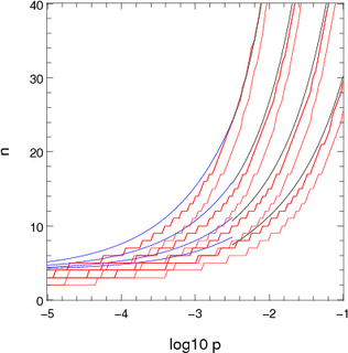Figure 1: Approximations used for computing the number of channels to consider stochastically when there is one dominant destination. The x-axis shows log10 p where p is the probability of not ending up in the dominant location. The pairs or red lines show the points where the chance of n channels not ending up in the dominant destination are 10-5 and 10-7. The blue and black lines show the two appoximations presented in the text. The different sets of lines correspond to different population sizes: 2000 (top set), 700, 250 and 100 (bottom set).

Future considerations

A second approach is to first generate the number of channels that do not end up in the preferred state, and then to allocate states randomly for just those. For large populations the process can be repeated: of those that do change, generate the number that do not end up in the most popular destination state and then allocate the rest randomly among the remaining states. This cuts down on the use of random numbers to compute destination states but part of the benefit is lost through the more complex statistics needed to generate the number of channels changing state. Blackwell proposed a method for stochastic diffusion that uses precomputed lookup tables for binomial distributions. It economises on operations but requires more memory accesses. Currently, PSICS does not use a prcedure of this sort and the dividing lines where it would become more cost effective are not clear. However, since executing this algorithm is the dominant cost in most PSICS models, the fine details are likely to have a significant effect on overall performance. Optimizing methods of switching between the possible algorithms is likely to be the most fruitful research direction in which to find further performance gains.

Properties and benefits

One advantage of the simplicity of the algorithm for deterministic channels is that the results can be made to be smooth functions of the parameter values down to the machine precision even where they deviate from the "correct" solution by much more than that. This is because there are no conditional blocks, case statements or loop terminating conditions that depend on parameter values or on the progress of the solution. Given the structure of the model, the sequence of operations is exactly the same whatever the parameter values. This not normally the case for numerical solutions of differential equations which generally use different methods depending on parameter values, or implement stopping conditions that depend on the solution being computed.

The interest of this form of smoothness is that it allows accurate numerical derivatives to be computed using a parameter increment that is smaller than the absolute error in the result (in most cases a solution would be choppy on this scale so a larger increment or finer tolerance would be required). Derivatives are required for efficient optimization schemes used in model fitting and the ability to compute them accurately, even on scales where the absolute solution is not accurate, means that optimisation algorithms can be effectively applied even to relatively coarse models. Such models can be run much more quickly than if high precisin is required and the result is that PSICS forms a convenient and efficient way to compute error functions for use in fitting models to data.